Librosa库-语音信号处理
语音信号处理库——Librosa
librosa语音信号处理 - 简书 (jianshu.com)这篇文章说的非常详细,但有一些函数已经荒废了我做了一些补充。
librosa — librosa 0.8.1 documentation官方文档
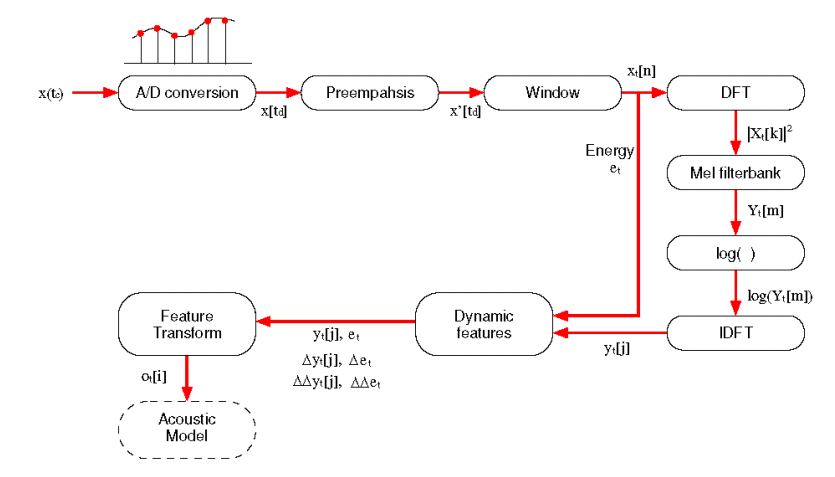
特征提取流程图:
1.读取语音
1 | y,sr = librosa.load(path, sr=22050, mono=True, offset=0.0, duration=None) |
参数:
- path:文件路径;
- sr:采样频率,默认22050,可以用参数’None’表示用原语音自身的采样频率;
- mono:是否将音频转换为单声道
- offset:表示音频读取的位置,以s为单位
- duration:表示读取音频的长度,以s为单位
返回值:
- y:音频时间序列
- sr:音频的采样频率
1 | import librosa |
2.读取时长
1 | d = librosa.get_duration(y=None, sr=22050, S=None, n_fft=2048, hop_length=512, center=True, filename=None) |
参数:
- y :音频时间序列
- sr :y的音频采样率
- S :STFT矩阵或任何STFT衍生的矩阵(例如,色谱图或梅尔频谱图)。根据频谱图输入计算的持续时间仅在达到帧分辨率之前才是准确的。如果需要高精度,则最好直接使用音频时间序列。
- n_fft :S的 FFT窗口大小
- hop_length :S列之间的音频样本数
- center :布尔值
- 如果为True,则S [:, t]的中心为y [t * hop_length]
- 如果为False,则S [:, t]从y[t * hop_length]开始
- filename :如果提供,则所有其他参数都将被忽略,并且持续时间是直接从音频文件中计算得出的。
返回值:
- d:音频时长
1 | librosa.get_duration(y,sr)#承接上面的代码 |
3.采样率
1 | sr = librosa.get_samplerate(path) |
参数:
- path:音频文件的路径
返回:
- sr:音频文件的采样率
1 | librosa.get_samplerate("test.wav") |
4.写音频
1 | #librosa.output.write_wav(path, y, sr, norm=False)在0.7.0版本荒废了现在要用soundfile.write() |
参数:
- file:要保存的文件名
- data:音频时间序列
- samplerate:音频的采样率
- 其他参数:参考SoundFile — PySoundFile 0.10.3post1-1-g0394588 documentation
1 | import soundfile as sf |
5.过零率
1 | zcr = librosa.feature.zero_crossing_rate(y, frame_length = 2048, hop_length = 512, center = True) |
参数:
- y :音频时间序列
- frame_length :帧长
- hop_length :帧移
- center:bool,如果为True,则通过填充y的边缘来使帧居中。
返回:
- zcr:zcr[0,i]是第i帧中的过零率
1 | librosa.feature.zero_crossing_rate(y) |
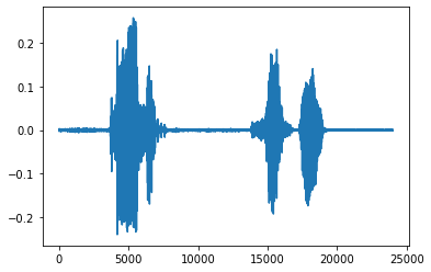
6.波形图
1 | librosa.display.waveplot(y, sr=22050, x_axis='time', offset=0.0, ax=None) |
参数:
- y :音频时间序列
- sr :y的采样率
- x_axis :str {‘time’,‘off’,‘none’}或None,如果为“时间”,则在x轴上给定时间刻度线。
- offset:水平偏移(以秒为单位)开始波形图
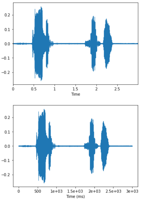
1 | #librosa.display.waveplot在0.9.0会废除,所以这里推荐使用librosa.display.waveshow |
参数:
- max_points:绘制的最大时间点数,如果超过持续时间,则执行下采样
- max_sr:可视化的最大采样率
1 | import librosa.display |
7.短时傅里叶变换
1 | D = librosa.stft(y,n_fft=2048,hop_length=None,win_length=None,window='hann',center=True,pad_mode='reflect') |
短时傅立叶变换(STFT),返回一个复数矩阵使得D(f,t)
- 复数的实部:np.abs(D(f,t))频率的振幅
- 复数的虚部:np.angle(D(f,t))频率的相位
参数:
-
y:音频时间序列
-
n_fft:FFT窗口大小,n_fft=hop_length+overlapping
-
hop_length:帧移,如果未指定,则默认win_length / 4。
-
win_length:每一帧音频都由window()加窗。窗长win_length,然后用零填充以匹配N_FFT。默认win_length=n_fft。
-
window
:字符串,元组,数字,函数 shape =(n_fft, )
- 窗口(字符串,元组或数字);
- 窗函数,例如scipy.signal.hanning
- 长度为n_fft的向量或数组
-
center
:bool
- 如果为True,则填充信号y,以使帧 D [:, t]以y [t * hop_length]为中心。
- 如果为False,则D [:, t]从y [t * hop_length]开始
-
dtype:D的复数值类型。默认值为64-bit complex复数
-
pad_mode:如果center = True,则在信号的边缘使用填充模式。默认情况下,STFT使用reflection padding。
返回:
- STFT矩阵,
1 | librosa.stft(y,center=True) |
8.短时傅里叶逆变换
1 | y = librosa.istft(stft_matrix, hop_length=None, win_length=None, window='hann', center=True, length=None) |
短时傅立叶逆变换(ISTFT),将复数值D(f,t)频谱矩阵转换为时间序列y,窗函数、帧移等参数应与stft相同
参数:
-
stft_matrix :经过STFT之后的矩阵
-
hop_length :帧移,默认为
-
win_length :窗长,默认为n_fft
-
window
:字符串,元组,数字,函数或shape = (n_fft, )
- 窗口(字符串,元组或数字)
- 窗函数,例如scipy.signal.hanning
- 长度为n_fft的向量或数组
-
center:bool
- 如果为True,则假定D具有居中的帧
- 如果False,则假定D具有左对齐的帧
-
length:如果提供,则输出y为零填充或剪裁为精确长度音频
返回:
- y :时域信号
9.幅度转dB
1 | librosa.amplitude_to_db(S, ref=1.0) |
将幅度频谱转换为dB标度频谱。也就是对S取对数。与这个函数相反的是librosa.db_to_amplitude(S)
参数:
- S :输入幅度
- ref :参考值,振幅abs(S)相对于ref进行缩放,
返回:
- dB为单位的S
10.功率转dB
1 | librosa.core.power_to_db(S, ref=1.0) |
将功率谱(幅度平方)转换为分贝(dB)单位,与这个函数相反的是librosa.db_to_power(S)
参数:
- S:输入功率
- ref :参考值,振幅abs(S)相对于ref进行缩放,
返回:
- dB为单位的S
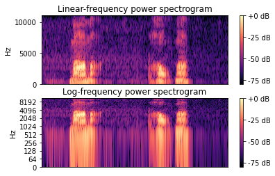
11.语谱图
1 | librosa.display.specshow(data, x_axis=None, y_axis=None, sr=22050, hop_length=512) |
参数:
- data:要显示的矩阵
- sr :采样率
- hop_length :帧移
- x_axis 、y_axis :x和y轴的范围
- 频率类型
- ‘linear’,‘fft’,‘hz’:频率范围由FFT窗口和采样率确定
- ‘log’:频谱以对数刻度显示
- ‘mel’:频率由mel标度决定
- 时间类型
- time:标记以毫秒,秒,分钟或小时显示。值以秒为单位绘制。
- s:标记显示为秒。
- ms:标记以毫秒为单位显示。
- 所有频率类型均以Hz为单位绘制
1 | #窗长大,窄带语谱图 |
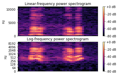
1 | #窗长减小,则是宽带语谱图 |
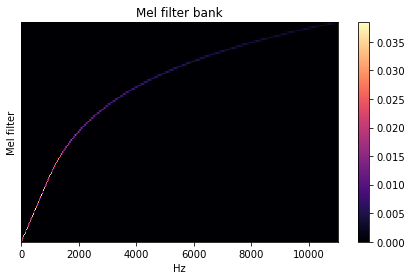
12.Mel滤波器组
1 | librosa.filters.mel(sr, n_fft, n_mels=128, fmin=0.0, fmax=None, htk=False, norm=1) |
创建一个滤波器组矩阵以将FFT合并成Mel频率
参数:
-
sr :输入信号的采样率
-
n_fft :FFT组件数
-
n_mels :产生的梅尔带数
-
fmin :最低频率(Hz)
-
fmax:最高频率(以Hz为单位)。如果为None,则使用fmax = sr / 2.0
-
norm
:{None,1,np.inf} [标量]
- 如果为1,则将三角mel权重除以mel带的宽度(区域归一化)。否则,保留所有三角形的峰值为1.0
返回:
- Mel变换矩阵
1 | melfb = librosa.filters.mel(22050, 2048) |
13.计算Mel scaled 频谱
1 | librosa.feature.melspectrogram(y=None, sr=22050, S=None, n_fft=2048, hop_length=512, win_length=None, window='hann', center=True, pad_mode='reflect', power=2.0) |
如果提供了频谱图输入S,则通过mel_f.dot(S)将其直接映射到mel_f上。
如果提供了时间序列输入y,sr,则首先计算其幅值频谱S,然后通过mel_f.dot(S ** power)将其映射到mel scale上 。默认情况下,power= 2在功率谱上运行。
参数:
-
**y **:音频时间序列
-
**sr **:采样率
-
**S **:频谱
-
**n_fft **:FFT窗口的长度
-
**hop_length **:帧移
-
**win_length **:窗口的长度为win_length,默认
win_length = n_fft -
**window **:字符串,元组,数字,函数或shape =(n_fft, )
- 窗口规范(字符串,元组或数字);看到scipy.signal.get_window
- 窗口函数,例如 scipy.signal.hanning
- 长度为n_fft的向量或数组
-
center
:bool
- 如果为True,则填充信号y,以使帧 t以y [t * hop_length]为中心。
- 如果为False,则帧t从y [t * hop_length]开始
-
power:幅度谱的指数。例如1代表能量,2代表功率,等等
-
n_mels:滤波器组的个数 1288
-
fmax:最高频率
返回:
- Mel频谱shape=(n_mels, t)
1 | import librosa.display |
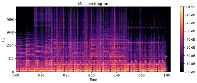
14.提取Log-Mel Spectrogram 特征(FBank特征)
1 | import librosa |
可见,Log-Mel Spectrogram特征是二维数组的形式,128表示Mel频率的维度(频域),64为时间帧长度(时域),所以Log-Mel Spectrogram特征是音频信号的时频表示特征。其中,n_fft指的是窗的大小,这里为1024;hop_length表示相邻窗之间的距离,这里为512,也就是相邻窗之间有50%的overlap;n_mels为mel bands的数量,这里设为128。
15.提取MFCC系数
1 | librosa.feature.mfcc(y=None, sr=22050, S=None, n_mfcc=20, dct_type=2, norm='ortho', **kwargs) |
参数:
- y:音频数据
- sr:采样率
- S:np.ndarray,对数功能梅尔谱图
- n_mfcc:int>0,要返回的MFCC数量
- dct_type:None, or {1, 2, 3} 离散余弦变换(DCT)类型。默认情况下,使用DCT类型2。
- norm: None or ‘ortho’ 规范。如果dct_type为2或3,则设置norm =’ortho’使用正交DCT基础。 标准化不支持dct_type = 1。
返回:
- M: MFCC序列
1 | import librosa |